Prediction API
This page documents how you can use OpenPifPaf from your own Python code. It focuses on single-image prediction. This API interface is for more advanced use cases. Please refer to Getting Started: Prediction for documentation on the command line interface.
import io
import numpy as np
import PIL
import requests
import torch

device = torch.device('cpu')
# device = torch.device('cuda')  # if cuda is available

print('OpenPifPaf version', openpifpaf.__version__)
print('PyTorch version', torch.__version__)
OpenPifPaf version 0.12.7+1.g0d67fa9
PyTorch version 1.7.1+cpu
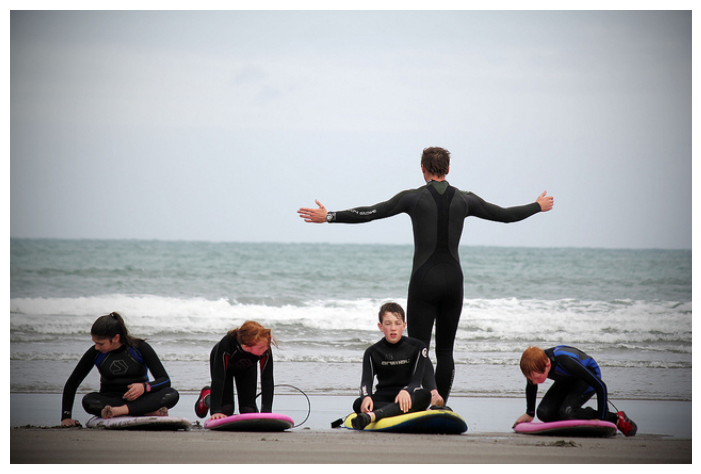
Load an Example Image
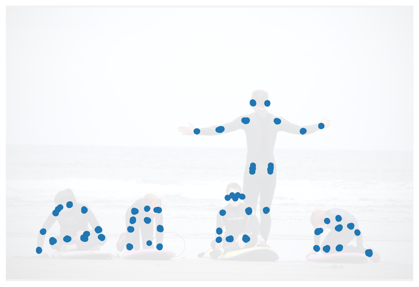
Image credit: “Learning to surf” by fotologic which is licensed under CC-BY-2.0.
image_response = requests.get('https://raw.githubusercontent.com/vita-epfl/openpifpaf/main/docs/coco/000000081988.jpg')
pil_im = PIL.Image.open(io.BytesIO(image_response.content)).convert('RGB')
im = np.asarray(pil_im)

with openpifpaf.show.image_canvas(im) as ax:
    pass
Load a Trained Neural Network
net_cpu, _ = openpifpaf.network.Factory(checkpoint='shufflenetv2k16', download_progress=False).factory()
net = net_cpu.to(device)
decoder = openpifpaf.decoder.factory([hn.meta for hn in net_cpu.head_nets])
Preprocessing, Dataset
Specify the image preprocossing. Beyond the default transforms, we also use CenterPadTight(16) which adds padding to the image such that both the height and width are multiples of 16 plus 1. With this padding, the feature map covers the entire image. Without it, there would be a gap on the right and bottom of the image that the feature map does not cover.
preprocess = openpifpaf.transforms.Compose([
    openpifpaf.transforms.NormalizeAnnotations(),
    openpifpaf.transforms.CenterPadTight(16),
    openpifpaf.transforms.EVAL_TRANSFORM,
])
data = openpifpaf.datasets.PilImageList([pil_im], preprocess=preprocess)
Dataloader, Visualizer
loader = torch.utils.data.DataLoader(
    data, batch_size=1, pin_memory=True,
    collate_fn=openpifpaf.datasets.collate_images_anns_meta)

annotation_painter = openpifpaf.show.AnnotationPainter()
Prediction
for images_batch, _, __ in loader:
    predictions = decoder.batch(net, images_batch, device=device)[0]
    with openpifpaf.show.image_canvas(im) as ax:
        annotation_painter.annotations(ax, predictions)
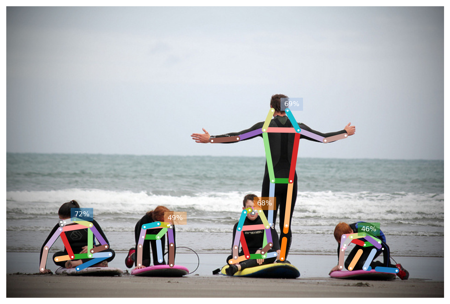
Each prediction in the predictions list above is of type Annotation. You can access the joint coordinates in the data attribute. It is a numpy array that contains the \(x\) and \(y\) coordinates and the confidence for every joint:
predictions[0].data
array([[ 81.05422   , 319.75046   ,   0.76443654],
       [ 85.04521   , 316.01663   ,   0.8613466 ],
       [ 79.32331   , 315.25885   ,   0.50764793],
       [ 99.83703   , 312.39368   ,   0.91851234],
       [  0.        ,   0.        ,   0.        ],
       [122.562065  , 319.91125   ,   0.833035  ],
       [ 78.57219   , 326.5119    ,   0.827177  ],
       [145.52835   , 351.6458    ,   0.84586245],
       [ 57.84586   , 354.2724    ,   0.77354056],
       [125.43357   , 358.20248   ,   0.7466016 ],
       [ 51.845222  , 384.3738    ,   0.80854195],
       [122.16235   , 364.6663    ,   0.760463  ],
       [ 95.9382    , 366.63358   ,   0.77250606],
       [150.77545   , 363.01898   ,   0.70611745],
       [ 73.452385  , 370.07568   ,   0.70078737],
       [104.37232   , 383.81467   ,   0.5096796 ],
       [  0.        ,   0.        ,   0.        ]], dtype=float32)
Fields
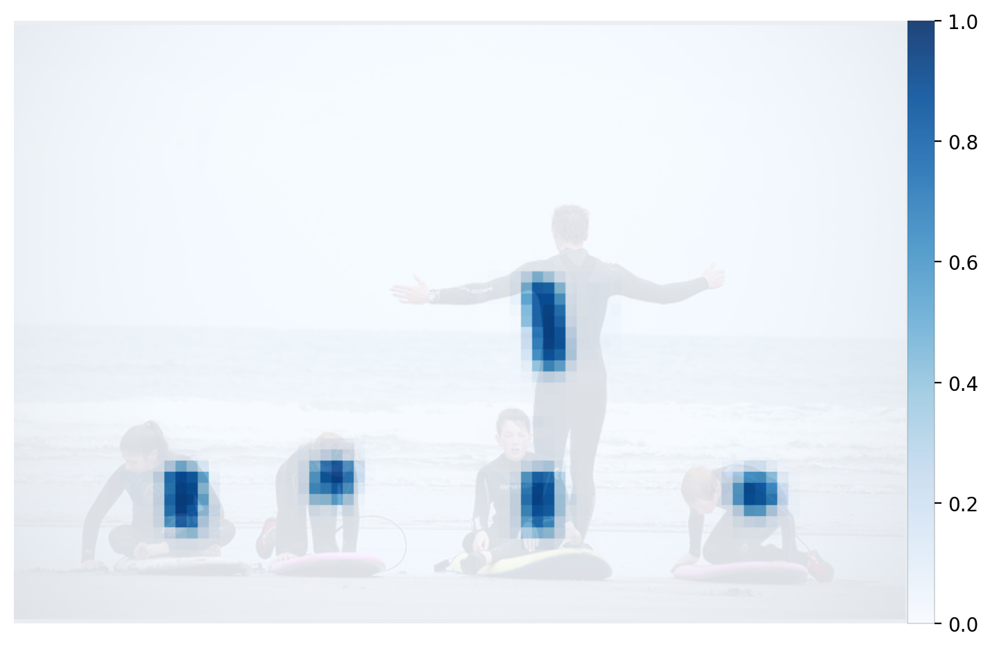
Below are visualizations of the fields. When using the API here, the visualization types are individually enabled. Then, the index for every field to visualize must be specified. In the example below, the fifth CIF (left shoulder) and the fifth CAF (left shoulder to left hip) are activated.
These plots are also accessible from the command line: use --debug-indices cif:5 caf:5 to select which joints and connections to visualize.
openpifpaf.visualizer.Base.set_all_indices(['cif,caf:5:confidence'])

for images_batch, _, __ in loader:
    predictions = decoder.batch(net, images_batch, device=device)[0]
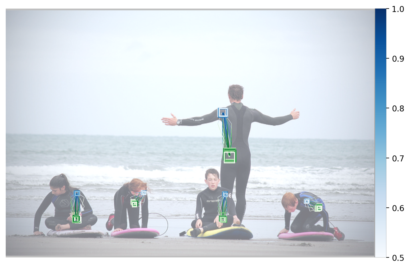
openpifpaf.visualizer.Base.set_all_indices(['cif,caf:5:regression'])

for images_batch, _, __ in loader:
    predictions = decoder.batch(net, images_batch, device=device)[0]
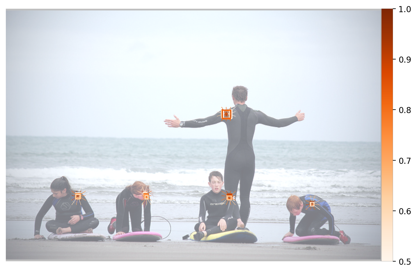
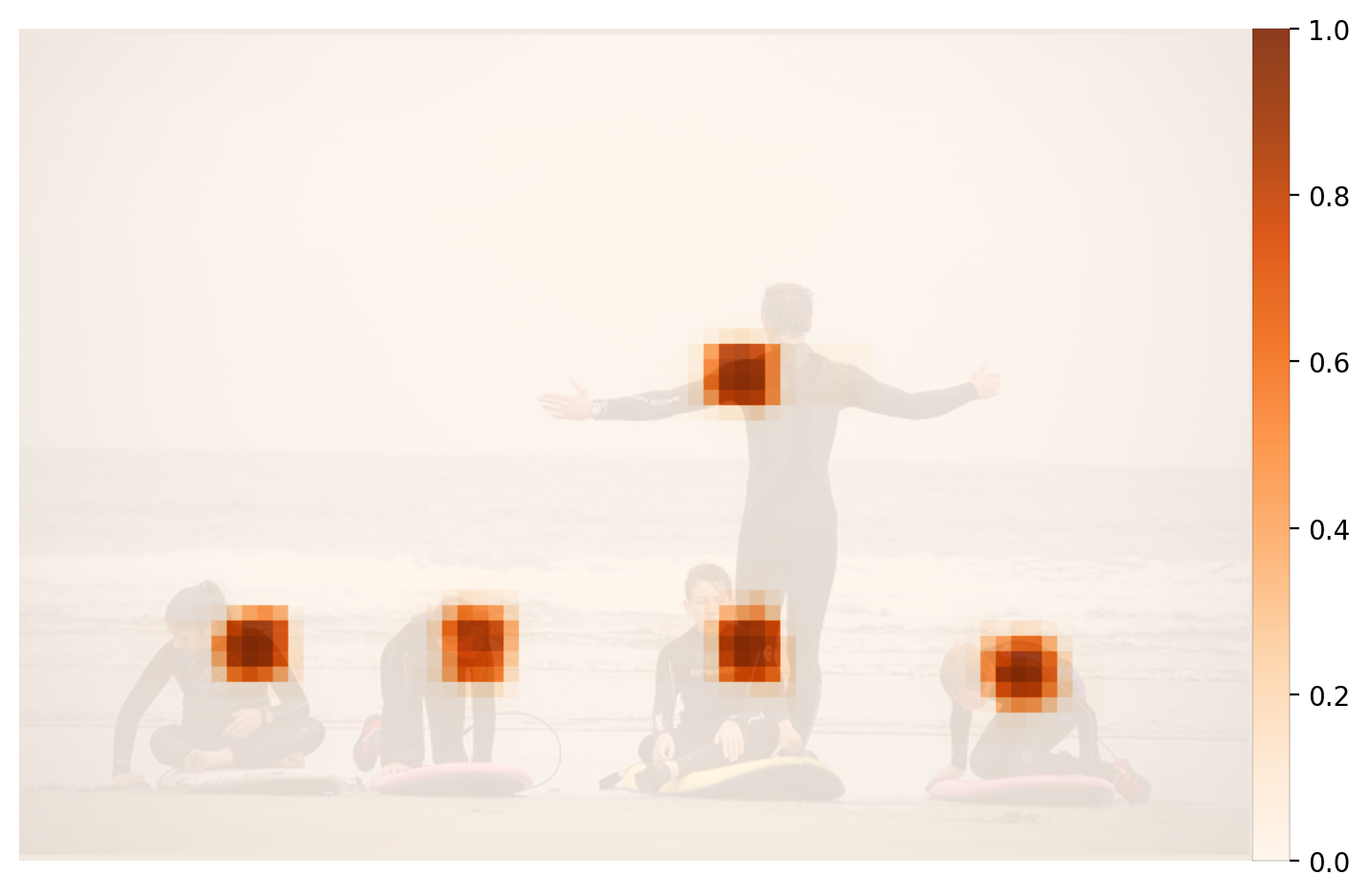
From the CIF field, a high resolution accumulation (in the code it’s called CifHr) is generated.
This is also the basis for the seeds. Both are shown below.
openpifpaf.visualizer.Base.set_all_indices(['cif:5:hr', 'seeds'])

for images_batch, _, __ in loader:
    predictions = decoder.batch(net, images_batch, device=device)[0]
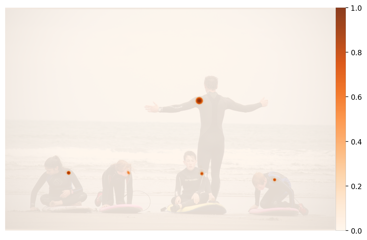
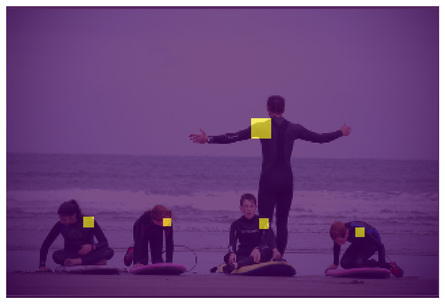
Starting from a seed, the poses are constructed. At every joint position, an occupancy map marks whether a previous pose was already constructed here. This reduces the number of poses that are constructed from multiple seeds for the same person. The final occupancy map is below:
openpifpaf.visualizer.Base.set_all_indices(['occupancy:5'])

for images_batch, _, __ in loader:
    predictions = decoder.batch(net, images_batch, device=device)[0]