Training¶

This section introduces training to create your own models. You don’t need to do this step if you use pre-trained models for Prediction on your own images. For training, you will need a dataset. See Datasets for instructions about a few popular datasets.

Training a model can take several days even with a good GPU. Many times existing models can be refined to avoid training from scratch.

The main interface for training with OpenPifPaf is the command line tool openpifpaf.train. A quick way to get started is with the training commands of the pre-trained models. The exact training command that was used for a model is in the first line of the training log file. Below are a few examples for various backbones.

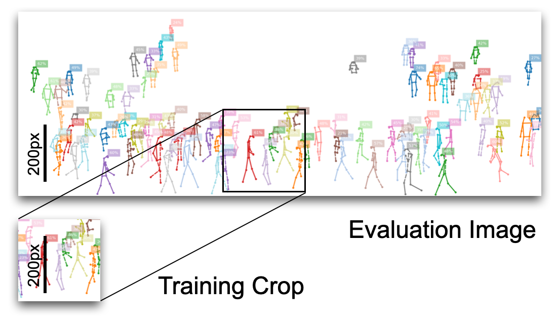
Training Crop Size¶

Training and evaluation image sizes are unrelated in fully convolutional architectures like OpenPifPaf. Instance size distribution between training and evaluation needs to be preserved. The size of the image that surrounds the instance to detect has little impact: for humans of height 100px, it does not matter whether that is inside a \(640\times480\) image or inside a 4k or 8k image. Therefore, you can keep the size of your training crops (selected with --square-edge) quite small even when evaluating on large images. The default is --square-edge=385 for cocokp and that is reasonable when most of the humans are not larger than 300px during evaluation. training crop size

The training crop size is a major factor for GPU memory consumption and for training time.

Reproducibility¶

Every training log file contains the command that was used to train under the key args. There is also a version key that specifies the precise version of OpenPifPaf that was used to train, like “0.11.9+204.g987345” (generated by versioneer). This means that the last tag was 0.11.9, that there are 204 additional commits beyond that tag, and that the hash of the current commit is “987345” (without the “g” as that simply stands for git). If you had uncommitted changes, there is an additional “dirty” suffix. Try to avoid “dirty” version numbers for training as it is impossible to tell whether you were just correcting a typo in the readme or had a substantial change that influences the training. Your local git command line client but also GitHub can compare to the short git hashes.

Multiple Datasets¶

OpenPifPaf supports simultaneous training on multiple datasets. You specify multiple datasets by concatenating them with a -, e.g. to train on COCO Keypoints cocokp and on COCO Detections cocodet you specify in your training command --dataset=cocokp-cocodet. This also works for custom datasets defined in plugins.

The samples from each dataset are tracked with weighted counters and the dataset for the next batch is chosen by the lowest counter. You specify the dataset weights (or you can think of it as an importance), for example, as --dataset-weights 1.0 0.5. That means that the first dataset (cocokp in the above example) is twice as important as the second one (e.g. cocodet) and two-thirds of the batches will be from the first dataset and one-third will be from the second.

An epoch is over once the first of the datasets is out of samples. As the datasets are randomized during training, a different set of samples will be used from epoch to epoch. That means that eventually all data will be utilized of the larger datasets even if not all data is used during a single epoch.

Overfitting¶

An effective way to validate the pipeline is working, loss functions are implemented correctly, encoders are correct, etc. is to overfit on a single image. You should be able to produce perfect predictions for that image. Some caveats: you need to deactivate augmentations, you must evaluate at the exact trained image size and the image should not contain crowd annotations (i.e. areas that will be ignored during training). Here is an example training command for a cocokp overfitting experiment:

time CUDA_VISIBLE_DEVICES=1 python3 -m openpifpaf.train \
  --lr=0.01 --momentum=0.9 --b-scale=5.0 \
  --epochs=1000 --lr-warm-up-epochs=100 \
  --batch-size=4 --train-batches=1 --val-batches=1 --val-interval=100 \
  --weight-decay=1e-5 \
  --dataset=cocokp --cocokp-upsample=2 --cocokp-no-augmentation \
  --basenet=shufflenetv2k16

The very first image in the training set has a large crowd annotation. Therefore, the above command overfits on four images. Here is the corresponding predict command for the second image in the training set:

python3 -m openpifpaf.predict \
  --checkpoint outputs/shufflenetv2k16-201007-153356-cocokp-1de9503b.pkl \
  --debug-indices cif:5 caf:5 --debug-images --long-edge=385 --loader-workers=0 \
  --save-all --image-output all-images/overfitted.jpeg \
  data-mscoco/images/train2017/000000262146.jpg

While the field predictions are almost perfect, it will predict two annotations while there is only one ground truth annotation. That is because the standard skeleton has no connection that goes directly from left-ear to nose and the left-eye is not visible and not annotated. You can add --dense-connections to include additional connections in the skeleton which will connect the nose keypoint to the rest of the skeleton.

ShuffleNet¶

ShuffleNet models are trained without ImageNet pretraining:

time CUDA_VISIBLE_DEVICES=0,1 python3 -m openpifpaf.train \
  --lr=0.0003 --momentum=0.95 --b-scale=10.0 --clip-grad-value=10 \
  --epochs=250 --lr-decay 220 240 --lr-decay-epochs=10 \
  --batch-size=32 \
  --weight-decay=1e-5 \
  --dataset=cocokp --cocokp-upsample=2 --cocokp-extended-scale --cocokp-orientation-invariant=0.1 \
  --basenet=shufflenetv2k16

You can refine an existing model with the --checkpoint option. We found that for stable training, the learning rate \(\lambda\), the clip-grad-value \(c\) and the \(\epsilon\) from the denominator of the BatchNorm should obey:

(1)¶\[\begin{align} \lambda \cdot c &\leq \sqrt{\epsilon} \end{align}\]

where the default \(\epsilon\) is \(10^{-4}\) (different from the PyTorch default). To fit large models in your GPU memory, reduce the batch size and learning rate by the same factor.

ResNet¶

ResNet models are initialized with weights pre-trained on ImageNet. That makes their training characteristics different from ShuffleNet (i.e. they look great at the beginning of training).

Debug Plots¶

As for all commands, you need to decide whether you want to interactively show the plots in matplotlib with --show (I use itermplot) or to save image files with --save-all (defaults to the all-images/ directory).

You can inspect the ground truth fields that are used for training. Add --debug-images to activate all types of debug plots and, for example, select to visualize field 5 of CIF and field 5 of CAF with --debug-indices cif:5 caf:5.

You can run this on your laptop without a GPU. When debug is enabled, the training dataset is not randomized and therefore you only need the first few images in your dataset locally.

Logs¶

For reference, check out the log files of the pretrained models. Models with their log files are shared as release “Assets” in the separate openpifpaf-torchhub repository: click on “releases” and expand “Assets” on the latest release.

To visualize log files with openpifpaf.logs:

python3 -m openpifpaf.logs \
  outputs/resnet50block5-pif-paf-edge401-190424-122009.pkl.log \
  outputs/resnet101block5-pif-paf-edge401-190412-151013.pkl.log \
  outputs/resnet152block5-pif-paf-edge401-190412-121848.pkl.log

Evaluation metrics like average precision (AP) are created with the openpifpaf.eval tool. To produce evaluation metrics every five epochs for every new checkpoint that is created:

CUDA_VISIBLE_DEVICES=0 python3 -m openpifpaf.eval \
  --watch --checkpoint "outputs/shufflenetv2k??-*-cocokp*.pkl.epoch??[0,5]" \
  --loader-workers=2 \
  --decoder=cifcaf:0 \
  --dataset=cocokp --force-complete-pose --seed-threshold=0.2

Testset Submission¶

CUDA_VISIBLE_DEVICES=0 python3 -m openpifpaf.eval \
  --checkpoint shufflenetv2k30 \
  --loader-workers=2 \
  --decoder=cifcaf:0 \
  --dataset=cocokp --force-complete-pose --seed-threshold=0.2 \
  --cocokp-eval-testdev2017 --coco-no-eval-annotation-filter --write-predictions

This will produce the file shufflenetv2k30.eval-cocokp.zip which you can submit to the competition on codalab.

Detection (experimental)¶

time CUDA_VISIBLE_DEVICES=0,1 python3 -m openpifpaf.train \
  --lr=0.0003 --momentum=0.95 --clip-grad-value=10 \
  --epochs=150 \
  --lr-decay 130 140 --lr-decay-epochs=10 \
  --batch-size=64 \
  --weight-decay=1e-5 \
  --dataset=cocodet --cocodet-upsample=2 \
  --basenet=resnet18 --resnet-input-conv2-stride=2 --resnet-block5-dilation=2

with eval code:

CUDA_VISIBLE_DEVICES=0 python3 -m openpifpaf.eval \
  --watch --checkpoint "outputs/resnet??-*-cocodet*.pkl.epoch??[0,5]" \
  --loader-workers=2 \
  --dataset=cocodet --decoder=cifdet:0 \
  --seed-threshold=0.1 --instance-threshold=0.1

COCO AP=24.3% at epoch 90 (now outdated).

Cloud and HPC¶

OpenPifPaf can be trained on cloud infrastructure and in high performance computing (HPC) environments. We have good experience with the pytorch/pytorch docker containers. The latest tag does not include any development packages like gcc. For that, you need a “devel” package (e.g. pytorch/1.6.0-cuda10.1-cudnn7-devel).

This is a development flow that worked well for us:

start with an empty directory
launch the “devel” container and bind/link your current empty directory
create a Python virtualenv and install all software from within the devel container into the virtualenv
never modify this virtualenv from the host, always from within the devel container

After setting up your environment, you can execute the training. You can even use the container without the “devel” tools to submit the job.

HPC job submission: Our environment supports Slurm and Singularity. Run

sbatch ./train.sh \
  --lr=0.0003  # and all the other parameters for training from above

with train.sh containing:

#!/bin/bash -l
#SBATCH --nodes 1
#SBATCH --ntasks 1
#SBATCH --cpus-per-task 40
#SBATCH --mem 96G
#SBATCH --time 72:00:00
#SBATCH --account=<your-account-name>
#SBATCH --gres gpu:2

srun singularity exec --bind <make-host-dir-available> --nv pytorch_latest.sif \
  /bin/bash -c "source ./venv3/bin/activate && python3 -u -m openpifpaf.train $(printf '%q ' "$@")"

Similarly, an eval.sh script might be run with

sbatch ./eval.sh \
  --watch --checkpoint "outputs/shufflenetv2k16-201023-163830-cocokp.pkl.epoch??[0,5]" \
  --dataset=cocokp \
  --loader-workers=2 \
  --force-complete-pose --seed-threshold=0.2

and look like this:

#!/bin/bash -l
#SBATCH --nodes 1
#SBATCH --ntasks 1
#SBATCH --cpus-per-task 20
#SBATCH --mem 48G
#SBATCH --time 06:00:00
#SBATCH --account=<your-account-name>
#SBATCH --gres gpu:1

pattern=$1
shift

srun singularity exec --bind <make-host-dir-available> --nv pytorch_latest.sif \
  /bin/bash -c "source ./venv3/bin/activate && python3 -m openpifpaf.eval $(printf '%q ' "$@")"

DistributedDataParallel¶

This mode of parallelization is activated with the --ddp argument. With torch.distributed.launch:

python -m torch.distributed.launch \
  -m openpifpaf.train --ddp \
  --all-other-args

By default, this will replace all BatchNorms in the model with SyncBatchNorms. The only argument that behaves differently is --batch-size which is the total batch size across all GPUs with DataParallel but here with DistributedDataParallel it is the batch size of a single process/GPU. This is the behavior of PyTorch in these two modes and we did not add any code to change that. On SLURM, the equivalent sbatch script is:

#!/bin/bash -l
#SBATCH --ntasks 4
#SBATCH --cpus-per-task 20
#SBATCH --mem 48G
#SBATCH --time 72:00:00
#SBATCH --gres gpu:2  # or as many GPUs as you have in a node

srun --gpu-bind=closest singularity exec --bind /scratch/izar --nv pytorch_latest.sif \
  /bin/bash -c "source ./venv3/bin/activate && MASTER_ADDR=$(hostname) MASTER_PORT=7142 python3 -u -m openpifpaf.train --ddp $(printf "%s " "$@")"

OpenPifPaf Guide DEV