Prediction API

This page documents how you can use OpenPifPaf from your own Python code. It focuses on single-image prediction. This API interface is for more advanced use cases. Please refer to Getting Started: Prediction for documentation on the command line interface.

import io
import numpy as np
import PIL
import requests
import torch

print('OpenPifPaf version', openpifpaf.__version__)
print('PyTorch version', torch.__version__)

OpenPifPaf version 0.13.11
PyTorch version 1.13.1+cpu

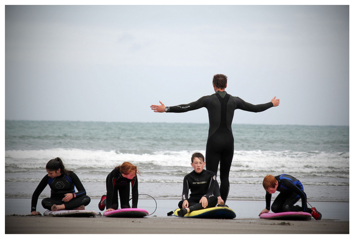
Load an Example Image

Image credit: “Learning to surf” by fotologic which is licensed under CC-BY-2.0.

image_response = requests.get('https://raw.githubusercontent.com/openpifpaf/openpifpaf/main/docs/coco/000000081988.jpg')
pil_im = PIL.Image.open(io.BytesIO(image_response.content)).convert('RGB')
im = np.asarray(pil_im)

with openpifpaf.show.image_canvas(im) as ax:
    pass

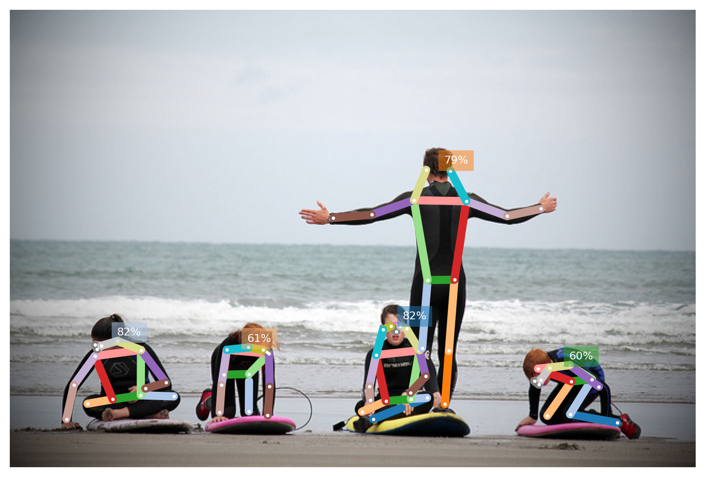
Use the Predictor API

predictor = openpifpaf.Predictor(checkpoint='shufflenetv2k16')
predictions, gt_anns, image_meta = predictor.pil_image(pil_im)

We can immediately visualize the predicted annotations (predictions):

annotation_painter = openpifpaf.show.AnnotationPainter()
with openpifpaf.show.image_canvas(im) as ax:
    annotation_painter.annotations(ax, predictions)

Each prediction in the predictions list above is of type Annotation. You can access the joint coordinates in the data attribute. It is a numpy array that contains the \(x\) and \(y\) coordinates and the confidence for every joint:

predictions[0]

<openpifpaf.annotation.Annotation at 0x7fbfe53dee20>

predictions[0].data

array([[ 3.6017877e+02,  2.9964966e+02,  9.9882096e-01],
       [ 3.6403537e+02,  2.9479474e+02,  9.5608473e-01],
       [ 3.5507379e+02,  2.9503970e+02,  9.7657114e-01],
       [ 3.6957544e+02,  2.9712769e+02,  8.2811129e-01],
       [ 3.4776544e+02,  2.9803622e+02,  9.4151646e-01],
       [ 3.8178815e+02,  3.1739853e+02,  9.3542975e-01],
       [ 3.4123145e+02,  3.2181036e+02,  9.5376050e-01],
       [ 3.8760934e+02,  3.4162189e+02,  6.1718684e-01],
       [ 3.3507935e+02,  3.5091327e+02,  9.6102822e-01],
       [ 3.7334406e+02,  3.5688290e+02,  4.3559963e-01],
       [ 3.3581897e+02,  3.6386734e+02,  8.9591628e-01],
       [ 3.7379721e+02,  3.6283130e+02,  8.5838985e-01],
       [ 3.5045963e+02,  3.6485587e+02,  9.5851350e-01],
       [ 3.8885754e+02,  3.6172189e+02,  6.5838528e-01],
       [ 3.2807568e+02,  3.7470078e+02,  6.8846005e-01],
       [ 3.3847418e+02,  3.8157928e+02,  3.4105796e-01],
       [ 0.0000000e+00, -3.0000000e+00,  0.0000000e+00]], dtype=float32)

The Predictor class can also be created with json_data=True and then it will return JSON serializable dicts and list instead of Annotation objects.

The other items that are returned are ground truth annotations (gt_anns) which are not provided for this image and meta information about the image (image_meta) which is useful to understand the transformations that were applied before passing the image through the neural network. Usually, you don’t need image_meta as the inverse transform has already been applied to ground truth and predictions in the Predictor class:

gt_anns

[]

image_meta

{'dataset_index': 0,
 'offset': array([ 0., -3.]),
 'scale': array([1., 1.]),
 'rotation': {'angle': 0.0, 'width': None, 'height': None},
 'valid_area': array([  0.,   3., 639., 426.]),
 'hflip': False,
 'width_height': array([640, 427])}

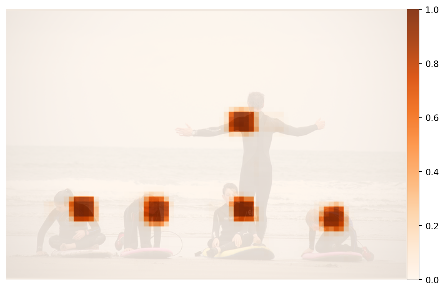
Fields

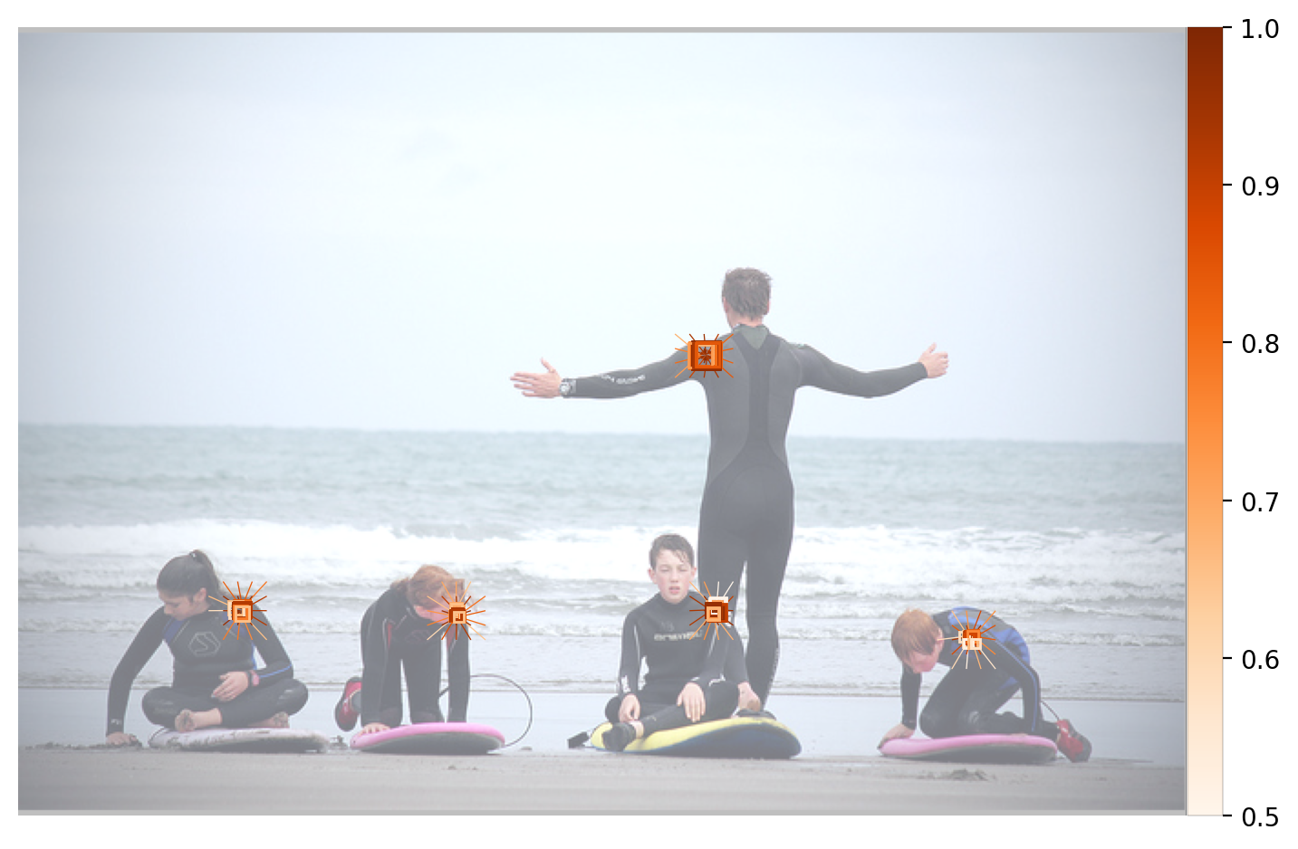
Below are visualizations of the fields. When using the API here, the visualization types are individually enabled. Then, the index for every field to visualize must be specified. In the example below, the fifth CIF (left shoulder) and the fifth CAF (left shoulder to left hip) are activated.

These plots are also accessible from the command line: use --debug-indices cif:5 caf:5 to select which joints and connections to visualize.

openpifpaf.visualizer.Base.set_all_indices(['cif,caf:5:confidence'])
_ = predictor.pil_image(pil_im)

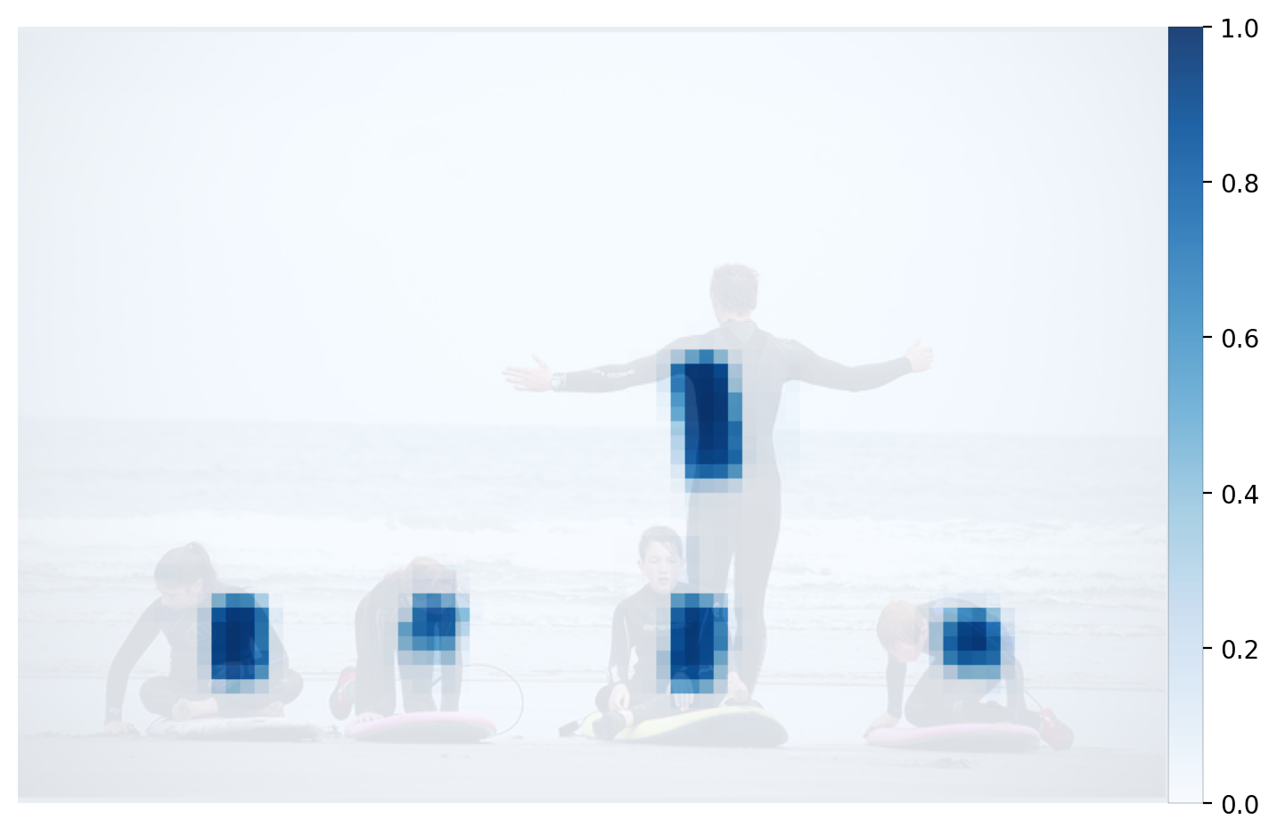
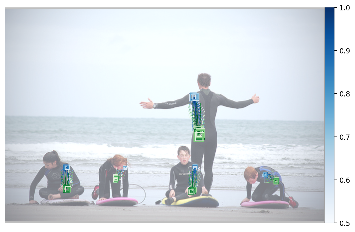
openpifpaf.visualizer.Base.set_all_indices(['cif,caf:5:regression'])
_ = predictor.pil_image(pil_im)

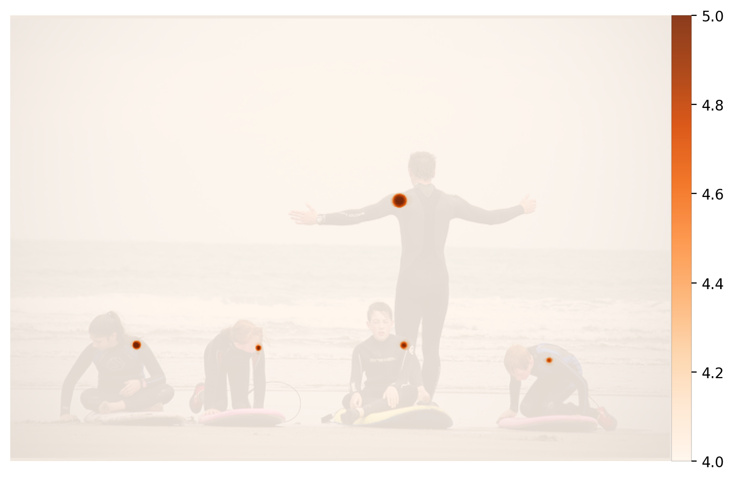
From the CIF field, a high resolution accumulation (in the code it’s called CifHr) is generated. This is also the basis for the seeds. Both are shown below.

openpifpaf.visualizer.Base.set_all_indices(['cif:5:hr', 'seeds'])
_ = predictor.pil_image(pil_im)

Starting from a seed, the poses are constructed. At every joint position, an occupancy map marks whether a previous pose was already constructed here. This reduces the number of poses that are constructed from multiple seeds for the same person. The final occupancy map is below:

openpifpaf.visualizer.Base.set_all_indices(['occupancy:5'])
_ = predictor.pil_image(pil_im)